Carbon analysis in BIM is difficult because the calculation itself is only one part of the problem.

The harder part is usually deciding where the assumptions live, how they connect to the model, and how much control the project team keeps while the workflow becomes repeatable.

This guide shows one practical way to run lifecycle assessment calculations in Vyssuals: keep the LCA assumptions in an external build-up table, join that table to Revit model data, calculate the global warming potential per element, and use the results for model analysis.

The Core Decision: Materials or Types

When you want to calculate embodied carbon from a Revit model, you usually have two options.

The first option is to calculate from the material layers already stored in the model. This can work well in later project stages, especially when the model is carefully maintained and you trust the material layers in walls, floors, roofs, doors, and families.

The second option is to calculate from Revit types. For early stage analysis, this is often the more practical path. Instead of relying on every material layer being perfectly modeled, you take a quantity from the model and multiply it by a unit rate for the relevant type.

For example:

Wall area multiplied by a GWP value per square meter
Railing length multiplied by a GWP value per meter
Door count multiplied by a GWP value per piece

This is where external build-up tables become useful.

What a Build-Up Table Does

A build-up table is an external source of LCA assumptions. It defines the carbon value for each model type or classification bucket outside the Revit file.

At minimum, the table needs three pieces of information:

Match key: the value used to connect the table row to Revit data, such as a type name or classification parameter
Base unit: the quantity basis for the calculation, such as m2, m, or pcs
GWP per unit: the global warming potential value for one unit of that type

For a wall, one build-up row might represent the full assembly per square meter: structural concrete, reinforcement, insulation, and cladding. For a door, one row might represent the full door assembly per piece. For a railing, one row might represent one linear meter.

The important part is that these assumptions do not need to live directly in Revit. They can be curated by a sustainability team, built from a national data source, reused across projects, or adjusted for one specific project.

Choosing a Matching Strategy

There are two useful matching patterns.

Match by Revit Type Name

Matching by type name gives you fine-grained control. Each Revit type can have its own build-up row and its own carbon value.

This is a good option when your type names are reliable and descriptive. It also works well when you want a close connection between model types and LCA assumptions.

Match by Classification Bucket

The other option is to match by a broader classification value.

Instead of mapping every wall type separately, you might group elements into buckets such as exterior walls, interior walls, structural floors, floor finishes, exterior doors, and railings. This does not mean grouping the elements in Revit. It means using model data to connect many elements to a shared LCA assumption.

This can be easier to maintain when the model is in an early design stage or has too many types for detailed matching.

From Material Data to Build-Up Unit Rates

It is useful to separate two different layers of information.

The first layer is material-level ground truth. This is where sources such as Oekobaudat, KBOB, LCAbyg, or an internal sustainability database are useful. They provide environmental data for individual materials or products, usually with values for phases such as A1 to A3.

The second layer is the build-up unit rate. This is the layer used by the workflow in this article. A build-up unit rate aggregates multiple material assumptions into one value for a whole Revit type or classification bucket.

For example, an exterior wall build-up might combine:

Structural concrete
Reinforcement
Insulation
Cladding
Interior finish

Those material-level values are then converted into one GWP value per square meter of that wall type. A door build-up might become one GWP value per piece. A railing build-up might become one GWP value per meter.

So the material database is not the build-up table itself. It is one source used to create the build-up table.

The build-up unit rates can be created in several ways:

By a sustainability expert or internal specialist team
From a company standard library of typical assemblies
Manually for one project using known assemblies and material quantities
With AI assistance, using material data and BIM type exports as inputs, followed by human review

The type export should include as much reliable information as possible: type name, category, description, width, function, fire rating, comments, and any other classification data. Descriptive type names and type comments help a lot.

For AI-assisted build-ups, the useful pattern is to provide two inputs: the material-level source data and an export of the BIM types that need aggregated build-up unit rates.

An agent can then create draft build-up rows by type. A practical orchestration is to split the work by unit basis:

Area-based elements, such as walls, floors, and roofs
Length-based elements, such as railings
Piece-based elements, such as doors, windows, furniture, and equipment

This can produce a useful first version quickly, but it should still be treated as an estimate that needs review. The value is speed and structure, not magic certainty.

The Workflow in Practice

The important sequence is this: first you export useful model and type information, then you use that export to create the build-up table, and only then do you bring the finished build-up table back into Vyssuals for calculation.

That gives the workflow two phases.

Phase 1: Export Model Data for the Build-Up Table

Before the build-up table exists, you need to give the person or AI agent creating it a useful export from the model.

This export is not just a calculation input. It is the raw context used to decide what each build-up row should represent.

For each relevant type or element group, you should export as much reliable information as you have:

Revit type name or another match key
Category
Description or type comments
Width or thickness
Function, such as interior or exterior
Above-ground or below-ground information
Fire rating or other performance data
Any other classification data that helps explain what the type is

This is where good BIM data pays off. Descriptive type names and type comments help the build-up process produce better estimates, especially when the model does not yet contain trustworthy material layers.

The result of this phase is an external build-up table with match keys, base units, and GWP values per unit.

Phase 2: Bring the Build-Up Table Back Into the Graph

Once the build-up table exists, the graph workflow can calculate and analyze the results.

1. Collect the Calculation Inputs

Start by collecting the model quantities and fields needed for the actual calculation.

For each element, you typically need:

Revit type name or another match key
Area for area-based elements
Length for length-based elements
Category or another grouping field for analysis
Any destination parameter if you want to write results back to Revit

Because the workflow is table-based, you can collect all relevant categories in one model input instead of building separate calculation tables for every category.

2. Join the Build-Up Table to the Model

Bring the Excel build-up table into the graph and join it to the model input.

The join connects the Revit match key, such as the type name, to the matching column in the Excel table. After the join, every model element carries the external LCA information from the build-up table:

Base unit
GWP per unit
Any additional notes or classifications from the external table

This is the central move in the workflow. The model supplies quantities. The external table supplies assumptions. The graph connects them.

3. Calculate GWP per Element

Use an Add Columns node to create a temporary result column, then use a Formula node to calculate the GWP per element.

The logic is simple:

if base unit is m2:
  area * GWP per unit
else if base unit is m:
  length * GWP per unit
else:
  GWP per unit

In the graph, this can be expressed with a case when formula. That is cleaner than a long chain of nested if statements, and it can work with string values such as m2, m, and pcs.

Even though the build-up table is defined per type, the calculation runs per element after the join. That gives you both detailed element-level results and aggregated summaries.

Aggregating and Reviewing the Results

After the per-element calculation, you can use Group and Aggregate nodes to summarize the results.

Useful summaries include:

Total GWP by type
Total GWP by category
High-impact buckets by unit rate
Element-level hotspots by total calculated result

This makes the workflow useful both for high-level reporting and for model-based investigation. You can quickly see whether walls, doors, railings, or another category drive the result, then drill into the relevant elements.

Writing Results Back to Revit

For deeper analysis, it can be useful to write calculated values back into Revit.

In the example workflow, the calculated GWP per element value is rounded and written into an LCA result parameter. The Create Changes node compares the graph values with the current values in Revit, stages the proposed changes, and lets you approve them before sending anything back.

This review step matters. Carbon data is analytical data, and you want a clear checkpoint before overwriting model parameters.

There is one Revit-specific detail to be aware of: if the parameter needs to vary by group instance, an area-type parameter can be a practical workaround for storing numeric values across grouped elements. It is not conceptually elegant, but it can avoid group-related parameter limitations in Revit.

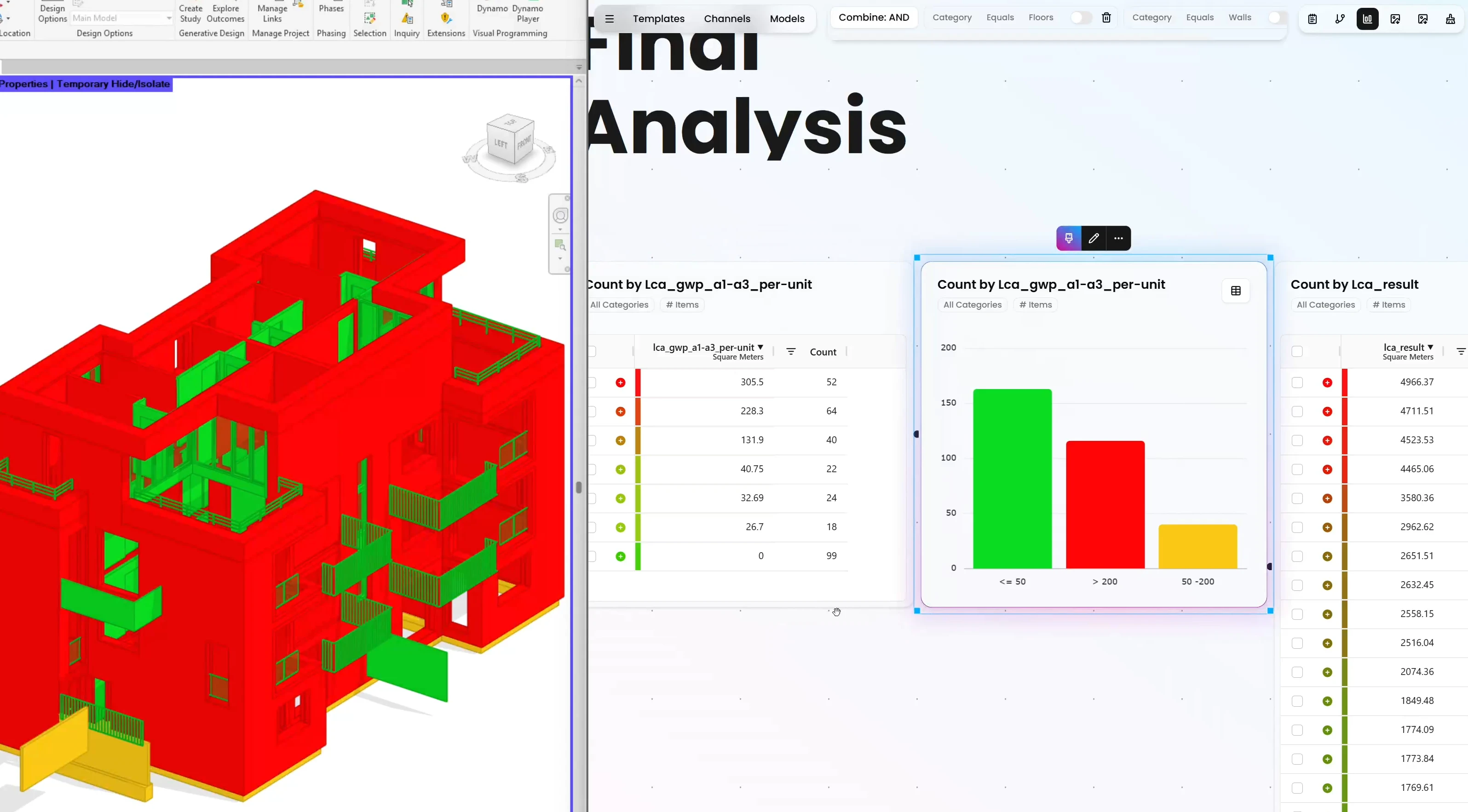
Visualizing Carbon in the Model

Once the result is available in the model or in the Vyssuals graph, you can visualize it in different ways.

One useful view is carbon intensity per unit. This helps identify which types have high GWP before element size is considered.

Another useful view is total GWP per element. This highlights the actual model hotspots. A very long wall may have a bigger total impact than a small element with a higher unit rate, simply because the quantity is larger.

Both views are useful. Unit-rate views help improve specifications. Total-result views help prioritize where the project impact actually sits.

Why This Is Better Than a One-Click Workflow

LCA is too assumption-heavy for a fully opaque one-click process.

A good workflow should automate the repetitive parts while keeping the assumptions visible:

Where did the GWP value come from?
What quantity basis was used?
Which model value was multiplied by which rate?
Which elements were included?
Which values were written back to Revit?

This approach gives you that control. The build-up table is external and reviewable. The graph is repeatable. The joins and formulas are visible. The results can be aggregated, visualized, and written back into the model when needed.

That balance is the point: enough automation to make carbon analysis practical, and enough control to keep the results trustworthy.

Want to see the workflow in action? Watch the walkthrough on our YouTube channel and get started with Vyssuals.